
Retail Velocity for Food and Beverage Brands: Separate Distribution Growth from More Units per Store
Learn how to calculate retail velocity, separate distribution gains from units per store, and decide where food and beverage media can improve sell-through.

· 14 min read
A beverage brand grows from 100 to 150 stores, then retail unit sales rise 25%. The rollout looks healthy, until the next report shows fewer units per store per week.
Surprisingly, both results can be correct.
Here's why. The original 100 stores sell more units per store than before, but the 50 newly added stores sell fewer units each, so they pull down the average across all 150 stores.
Total sales rise even as the blended rate falls.
To interpret that result, calculate sales against the right store exposure and compare stores present in both periods. Otherwise, expansion can look like weakening demand, while closing weak stores can make a shrinking business appear more productive.
For media planning, that distinction changes your next action.
Weak sales in newly stocked stores may call for a launch-support test; falling sales in established stores may require a stock, price or demand diagnosis first.
At 9AM, we start by checking availability and store-level performance, then test whether media can generate enough incremental contribution to cover its cost.
P.S. Our food and beverage retail media team can help connect that store-level picture to the next campaign decision.
What Does Retail Velocity Measure?
Retail velocity measures product sales relative to distribution over a defined period. Units per store per week (UPSPW) is useful for operational tracking within a comparable store group.
Some industry data providers also use distribution-weighted measures to account for differences in retailer size and assortment. ACV distribution shows what share of a retailer group's total sales volume sits in stores that carry your product, and total distribution points (TDP) add that up across your items. Neither tells you how fast the product sells once it is on shelf.
This guide uses units per live store-week, so compare only reports with the same store, SKU and period definitions.
Calculate Units per Store per Week From Store Exposure
Divide retail units sold by the store-weeks included in the report, using the same product and coverage rule throughout:
Operational UPSPW = retail units sold ÷ eligible live store-weeks
A store-week is one live store observed for one week. A store counts as live once the product is authorized and set up to sell there. Verified zero-sales weeks stay in the count, and so do stockout weeks, which you flag so you can compare the rate with and without them. Weeks with no report at all stay out.
With 100 stores live for four weeks, the denominator is 400 store-weeks.
If stores go live at different times, sum their actual eligible weeks instead of multiplying the final store count by the full period.
Pro tip: A data provider's 'stores selling' metric may exclude stores with zero sales, so label the metric before comparing it with this live-store rate.
Use consumer point-of-sale units to measure sell-through, meaning what shoppers actually buy.
Shipments into a distributor or retailer answer a different question: how much inventory entered the channel. They cannot establish how quickly shoppers bought it.
Also define the unit.
A case, multipack and individual can are different measures. Preserve the retailer's selling unit, or document the conversion before combining sources.
How Can Retail Sales Grow While Average Velocity Falls?
Retail sales can grow while average velocity falls when new distribution adds units at a lower sales rate than the existing footprint. The blended average changes even if retained stores, meaning the stores that sold the product in both periods, improve.
The same mix effect works in reverse: removing the slowest stores can raise average velocity while total sales fall.
Sally Martin's velocity Q&A explains both patterns.
The practical implication is to report retained stores separately, which the industry often calls same-store analysis, so a change in the store mix doesn't get mistaken for a change in their performance.
Separate Retained-Store Growth From New-Store Sales
Separate the units added by new stores from the change in stores present in both periods. The following illustration uses one beverage SKU over two equal four-week periods, with every included store live throughout its period.
There are no store exits, pack changes or missing weeks.
In the first period, 100 stores sell 2,400 units: 6 UPSPW. In the second, those same stores sell 2,600 units. Another 50 stores contribute 400 units.
The growth comes from two places:
200 additional units in retained stores: the same footprint sells more.
400 units in new stores: the expanded footprint adds business.
Together, that adds 600 units, taking total sales from 2,400 to 3,000.
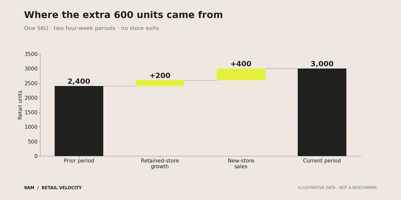
Figure 1. Reconcile the units before interpreting the average. Source: 9AM illustrative calculation; not a client result or category benchmark.
Now calculate the rates.
The current network has 600 store-weeks: 150 stores multiplied by four weeks. Its 3,000 units produce 5 UPSPW. Retained stores produce 6.5 UPSPW; new stores produce 2. To check it, weight the two groups by their size: (100 × 6.5 + 50 × 2) ÷ 150 = 5.0.
This is why the headline needs two rates and not just total sales. The same data produces the following results:
Signal | Prior period | Current period | Change |
|---|---|---|---|
Total retail units | 2,400 | 3,000 | +25% |
Stores live for the full period | 100 | 150 | +50% |
Network UPSPW | 6.0 | 5.0 | −16.7% |
Retained-cohort UPSPW | 6.0 | 6.5 | +8.3% |
The retained stores rise from 6 to 6.5 UPSPW (+8.3%), while the 50 new stores average only 2 UPSPW. Combining those groups yields 5 UPSPW across the expanded network, down from 6.
The lower network average therefore reflects the mix of new and retained stores instead of just weaker sales in the stores that were already carrying the product.
So what should the new stores be selling? The question for the rollout review is:
Are they following an acceptable ramp for that retailer, product and launch support?
Compare stores at similar weeks since launch.
A new-store group should not automatically inherit the mature-store target on its first trading week.
For example, a retailer might expect new stores to average about 2 UPSPW in their first four weeks and about 4 by week eight. If so, the 50 new stores are on track, even though they sit far below the 6.5 of the retained stores.
The retained-store improvement also needs context.
Promotions, price, availability and seasonality may explain some of it. A comparable cohort gives a cleaner description of what changed, but it does not prove what caused it.
What Should a Brand Check Before Spending on Media?
Verify the reported velocity drop. Build a view of retailer POS data by store, SKU and week, and use actual live store-weeks rather than the final store count. Keep verified zero-sales weeks, flag stockout weeks and leave out weeks with no report. A store that sold nothing is different from a store for which no data arrived.
Compare consistent store cohorts. Compare the same SKUs and selling units over equivalent periods. Check launch age, stockouts, price changes and promotions before attributing a slower rate to weaker shopper demand.
Choose the action that matches the diagnosis. The table below maps each pattern to its owner and next step. Media becomes a testable response only after those competing explanations have been checked.
Diagnose Distribution and Store-Level Sales Changes
Check data coverage and product availability first, then compare retained-store performance with the new-store ramp.
These checks distinguish a reporting or execution problem from a possible shopper-demand problem.
The table below maps each observed pattern to a diagnostic check, the team responsible and the action that follows.
Observed pattern | Checks before acting | Commercial owner | Next action |
|---|---|---|---|
Distribution rises; network velocity falls | Retained cohort, new-store age and store mix | Sales lead and analyst | Separate the ramp from mature-store performance |
Retained-cohort velocity falls | Price, promotions, stock and comparable periods | Sales, trade and marketing | Identify the changed condition before funding demand |
Velocity rises; distribution falls | Which stores exited and how they previously sold | Sales lead | Quantify lost units and the survivorship effect (the exited stores were probably the slow ones) |
Live stores show zero sales | Data completeness, shelf presence and inventory | Retailer or broker | Confirm execution and stock before activating media |
Velocity rises alongside stockouts | Available-to-sell inventory and replenishment | Supply and retailer teams | Restore purchase capacity; review media pacing |
Rule Out Execution First
Start with the operational constraint that could prevent a sale. A product may be authorized without being on the expected shelf, correctly priced or replenished. The retailer or broker usually needs to resolve those issues; a media partner can surface evidence and adjust spending around them.
Check promotion timing before interpreting stronger velocity as a response to advertising. If an offer ran during the campaign, the observed increase may reflect both activities, and the discount affects what the extra units contribute.
Connect the sales review to the trade-spend plan so media and promotion costs appear in the same commercial assessment.
Then Test the Demand Hypothesis
Once the product is actually available and the sales data is trustworthy, investigate why shoppers pass it over.
For example, if shoppers see an unfamiliar drink but cannot tell when to use it, a retailer-specific creative test could clarify its use occasion. If the issue is an uncompetitive shelf price, creative by itself is unlikely to fix the economics.
These remain hypotheses.
Isolate one intervention where possible and compare an appropriate control or baseline; a sales increase after changing creative does not, by itself, prove creative caused it.
Set an owner and a decision date for each intervention.
A broker shelf check, a replenishment fix and a creative test have different completion signals. Combining them into “improve velocity” makes accountability disappear.
Fixing a missing shelf placement can restore a purchase opportunity, while advertising cannot make an unavailable product purchasable. The retail media mistakes guide covers the cost of funding demand before those conditions are ready.
How Should Retail Velocity Guide Paid Media Investment?
Use retail velocity to choose which stocked markets to test, set the sales change the campaign should achieve and evaluate whether additional contribution covers its cost. The rate identifies where to investigate; a controlled test is needed to estimate what changed because of the media.
Fund Media Where the Product Can Be Purchased
Fund campaigns only where the advertised products are listed, live, and supported by credible availability data. Map those products and locations to the targeting controls available in the chosen account, so the campaign's reachable footprint matches the purchase opportunity.
For example, if a SKU is live in 60 of the 150 stores a regional campaign would cover, the campaign pays for impressions in the other 90 stores, where shoppers cannot buy it. Limiting the test to the 60 live stores keeps spend tied to a real purchase opportunity.
A launch-support test for new stores works the same way: run location-targeted ads around the 50 new stores and compare them with similar new stores that get no extra support.
For retail media, verify the account's product eligibility, retailer coverage and available targeting before designing the test.
For paid social or search, check location settings and the destination: a nearby shopper still needs a workable route to the stocked product.
Not every network supports store-level isolation or a clean holdout, meaning a group of stores deliberately left without ads.
This is where our F&B media buying team connects paid search, social and retail media to verified retail availability.
Set the test around a sales question the available retailer data and campaign controls can answer.
Test Whether Extra Sales Cover the Media Cost
Identify the incremental sales effect.
If feasible, compare similar stocked markets with and without the campaign, checking that their earlier sales patterns, prices and promotions were comparable.
Attribution reports which sales received ad credit; a credible comparison helps estimate how many sales were genuinely additional.
Compare exposed and unexposed stores.
Let’s suppose exposed stores improve from 5 to 6 units per store per week, while comparable unexposed stores improve from 5 to 5.5. The difference between those gains is 0.5 units per store per week. Analysts call this a difference-in-differences comparison.
This is only a plausible media effect if the groups would otherwise have followed similar trends and no other major condition changed. Our geo-lift guide explains how to build those comparison groups.
Now the question finance will ask: do the extra sales cover the media cost?
Across 100 exposed stores over four weeks, that estimated difference amounts to 200 additional units. Contribution per unit is what the brand keeps after retailer margin and variable costs, before media. At $1.40 per unit, they generate $280 toward media costs. If the campaign costs $500, it falls $220 short within the measurement window.
Pro tip: Our contribution margin guide shows how to calculate it.
That example is deliberately unprofitable to show why higher velocity alone is not enough to justify budget.
What Should a Buyer-Ready Retail Velocity Scorecard Include?
A buyer-ready scorecard should show both the growth story and its caveats, since the reader is usually the retailer's category buyer: total retail units, live store-weeks, network and retained-cohort UPSPW, new-store ramp, stock and promotion changes, and, only when supported by a credible test, incremental contribution.
Together, those measures explain where growth came from and what action the evidence supports.
Here is how the scorecard would read for the 100-to-150-store example:
Total retail units: 3,000, up 25% from 2,400.
Live store-weeks: 600 (150 stores × 4 weeks).
Network UPSPW: 5.0, down from 6.0.
Retained-cohort UPSPW: 6.5, up from 6.0.
New-store ramp: 2.0 UPSPW across 50 stores, to be compared with the retailer's expected ramp.
Stock and promotion changes: none recorded in this illustration.
Incremental contribution: not reported, because there is no controlled test yet.
Use a short operating sequence:
Validate the file and flag incomplete coverage.
Reconcile the unit bridge and the comparable cohorts.
Choose one intervention and write down its economic hypothesis.
Record the result, uncertainty and criteria for the next decision.
Use the weekly review to track execution and data completeness, with the final evaluation scheduled in advance.
Test length should follow the sales cycle, data lag and study design.
A new weekly report is not automatically enough evidence to change the investment decision.
Pro tip: keep a short decision log beside the scorecard that records what changed, which stores were affected, who approved the intervention and when to review the outcome.
If a launch expands during a test, document how the added stores enter the analysis.
This preserves the comparison rules when the next report arrives and helps a buyer distinguish observed progress from a revised measurement definition.
Improve Food and Beverage Sell-Through with 9AM
Adding stores is only the first step. The harder question is what each new store sells once it’s on the shelf, and whether a slower average points to a launch problem, a stock problem or a demand problem.
The cohort view answers that, by showing how retained stores perform and how new ones ramp.
At 9AM, we work with food and beverage brands as a long-term growth partner.
We start by validating your store list and POS baseline, then help you decide which stores need an execution fix and which are ready for media support.
As your distribution grows, we keep the scorecard current, so every new retailer or region comes with a ramp to compare against and a clear test of whether the extra sales cover their cost.
That keeps your sales, finance, and media teams working from one picture of what is selling, where, and why.
Book a strategy call to review your distribution file and recent POS data, and we’ll build a growth plan that keeps pace with your next rollout.
FAQs
What is a good units-per-store-per-week target for a beverage brand?
A useful target matches the retailer, category, pack, price tier and reporting period. Start with the buyer's verified requirement and comparable products under similar conditions. A 6-UPSPW target at a large grocery chain may be inappropriate for a small convenience-store account; there is no universal beverage threshold across formats and markets.
Should zero-sales stores be included in retail velocity?
Include valid zero-sales observations in the operational live-store view. A provider's selling-store metric may use a different denominator; show it separately and label it. Keep confirmed zero-sales weeks and flagged stockout weeks in the denominator; leave out weeks with no report.
Can brand velocity rise when individual SKUs weaken?
Yes, if the brand measure is units per store, adding more items can lift the total while an existing SKU slows. For example, if a brand launches a second flavor, units per store at brand level can rise while the first flavor slows because some shoppers switch to the new one. Compare brand-level movement with a stable SKU cohort, and check how assortment changes affect the base that the selected metric is divided by.
What can a brand measure with chain-level sales data only?
A brand can report chain-level sales trends and rates supported by available distribution data. It cannot establish retained-store performance without the relevant detail. Request store-level data or an appropriate syndicated breakdown before claiming same-store growth.
Does higher retail velocity prove repeat purchase?
No. POS units alone cannot distinguish more first-time buyers from more repeat purchases. Use household panel data or suitable customer-level purchase histories to measure repeat directly, rather than inferring it from the store sales rate.
About Mustafa Alkhtab
Mustafa Alkhtab is Head of Performance Media at inBeat Agency, where he oversees paid media and performance creative results across the agency's accounts. Before inBeat Agency, he built growth programs for ecommerce, lead generation, and mobile app businesses in international markets. He writes about media buying, measurement, and conversion rate optimization.
More from Mustafa AlkhtabKeep exploring.

Insights
Instacart Advertising for Food and Beverage Brands: What to Check Before Your First Campaign
November 12, 2026
Insights
Grocery Retail Media: How Food Brands Choose a Network Their Distribution Can Support
November 12, 2026

Insights
Amazon Fresh Advertising vs Amazon.com Ads: What Food Brands Must Verify Before Buying Media
November 12, 2026